Prong 1: Route Travelled & Dwell time by SSEC vessels
Exploring the routes travelled by SSEC vessels, we observed that while both vessels have overlapping paths (City of Lomark, Wrasse Bed, Ghoti Preserve), they travelled relatively separate routes.
Snapper Snatcher
Snapper Snatcher took a total of 19 trips from the 1 February 2035 to 14 May 2035, with an average trip duration of 5.3 days.
Peer Comparison on dwell time of vessel for similar size
Considering that the time a vessel is detected at an area is dependent on it’s length and speed to cover the area. We seek to understand if the dwell time of SSEC vessels are reasonable by comparing the vessels behaviour with other vessels of similar nature (Fishing vessels of relative length).
Out of the 178 fishing vessels, we observed that Snapper Snatcher (Red) is relatively small, whereas Roach Robber (Purple) is comparatively large. With distinct clusters by length, we subsequently compare the dwell time.
Code
N_vessel_fishing <- N_vessel %>%filter(vessel_type =="Fishing") %>%mutate(color =case_when( vessel_id =="snappersnatcher7be"~"red", vessel_id =="roachrobberdb6"~"purple",TRUE~"grey")) %>%mutate(tooltip_text =paste("Vessel name: ", vessel_name, "<br>","Vessel company: ", vessel_company, "<br>","Tonnage: ", tonnage, "<br>","Length: ", length_overall, "<br>" ))p <-ggplot(N_vessel_fishing, aes(x = length_overall, fill = color, text = tooltip_text)) +geom_histogram(bins =20, color ="black", alpha =0.7) +scale_fill_manual(values =c("grey"="grey", "red"="red", "purple"="purple")) +labs(title ="Histogram of Vessel Count per Overall Length", x ="Overall Length", y ="Vessel Count", fill ="Vessel") +theme(legend.position ="none") +theme_minimal()p_interactive <-ggplotly(p, tooltip ="text") %>%layout(title ="Histogram of Vessel Count per Overall Length") %>%layout(showlegend =FALSE)p_interactive
Code
# Create the second histogram based on tonnagep2 <-ggplot(N_vessel_fishing, aes(x = tonnage, fill = color, text = tooltip_text)) +geom_histogram(bins =30, color ="black", alpha =0.7) +scale_fill_manual(values =c("grey"="grey", "red"="red", "purple"="purple"))+labs(title ="Histogram of Vessel Count per Tonnage", x ="Tonnage", y ="Vessel Count", fill ="Vessel") +theme(legend.position ="none") +theme_minimal()p2_interactive <-ggplotly(p2, tooltip ="text") %>%layout(title ="Histogram of Vessel Count per Tonnage") %>%layout(showlegend =FALSE)p2_interactive
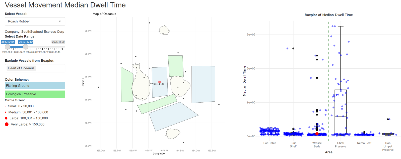
Out of the 178 fishing vessels, we identified 36 small vessels (Tonnage <= 800, Length <= 50) and 18 large vessels (Tonnage >= 9000, Length >= 110). Of which, we observed their dwell times for the fishing grounds and ecological preserve for the same time period where SSEC vessels were active. (1 February 2035 to 14 May 2035).
We observed that Snapper Snatcher has overstayed in multiple regions, Cod Table, and especially in Ghoti Reserve and Wrasse Beds. Meanwhile, Roach Robber has stayed largely in Wrasse Bed only, and have 2 notable instances of overstaying. Interestingly, large vessels such as Roach Robber do not stay long in Ghoti Preserve, and has not appeared in Don Limpet Preserve.
Code
# conditions, length <= 50, tonnage 800 - 36 vessels N_vessel_fishing_small <- N_vessel_fishing %>%filter(tonnage <=800, length_overall <=50)# conditions, length > 110 , tonnage >= 9,000 - 18 vesselsN_vessel_fishing_large <- N_vessel_fishing %>%filter(tonnage >=9000, length_overall >=110)ping_activity$start_time <-ymd_hms(ping_activity$start_time)# Define cutoff timecutoff_time <-ymd_hms("2035-05-14 00:00:00")# ping activity of small fishing vessel ping_activity_small <- ping_activity %>%filter(vessel_id %in% N_vessel_fishing_small$vessel_id, area %in%c("Cod Table", "Tuna Shelf", "Wrasse Beds", "Ghoti Preserve", "Nemo Reef", "Don Limpet Preserve"), start_time <= cutoff_time) %>%mutate(start_time_formatted =format(start_time, "%d-%m-%Y")) %>%mutate(color =case_when( vessel_id =="snappersnatcher7be"~"red", vessel_id =="roachrobberdb6"~"purple",TRUE~"grey" ))ping_activity_small <- ping_activity_small %>%mutate(tooltip_text =paste("Start Time: ", start_time_formatted, "<br>","Dwell: ", dwell, "<br>","Vessel ID: ", vessel_id, "<br>","Vessel Company: ", vessel_company ))p3 <-ggplot(ping_activity_small, aes(x = area, y = dwell, text = tooltip_text)) +geom_boxplot(outlier.shape =NA) +# Remove outliers since we'll show all points with jittergeom_jitter(aes(color = color), width =0.2, size =1.5, alpha =0.7) +# Add jitterscale_color_identity() +# Use the color values as islabs(title ="Boxplot of Dwell Time for Small Sized Fishing Vessels",x ="Area",y ="Dwell Time (seconds)") +theme_minimal()# Convert to plotly for interactivityp3_interactive <-ggplotly(p3, tooltip ="text")# repeat plot for large vesselping_activity_large <- ping_activity %>%filter(vessel_id %in% N_vessel_fishing_large$vessel_id, area %in%c("Cod Table", "Tuna Shelf", "Wrasse Beds", "Ghoti Preserve", "Nemo Reef", "Don Limpet Preserve"), start_time <= cutoff_time) %>%mutate(start_time_formatted =format(start_time, "%d-%m-%Y")) %>%mutate(color =case_when( vessel_id =="snappersnatcher7be"~"red", vessel_id =="roachrobberdb6"~"purple",TRUE~"grey" ))ping_activity_large <- ping_activity_large %>%mutate(tooltip_text =paste("Start Time: ", start_time_formatted, "<br>","Dwell: ", dwell, "<br>","Vessel ID: ", vessel_id, "<br>","Vessel Company: ", vessel_company ))p4 <-ggplot(ping_activity_large, aes(x = area, y = dwell, text = tooltip_text)) +geom_boxplot(outlier.shape =NA) +# Remove outliers since we'll show all points with jittergeom_jitter(aes(color = color), width =0.2, size =1.5, alpha =0.7) +# Add jitterscale_color_identity() +# Use the color values as islabs(title ="Boxplot of Dwell Time for Large Sized Fishing Vessels",x ="Area",y ="Dwell Time (seconds)") +theme_minimal()# Convert to plotly for interactivityp4_interactive <-ggplotly(p4, tooltip ="text")p3_interactive
Code
p4_interactive
Prong 2: Comparing the Mapped Cargo for SSEC Vessels.
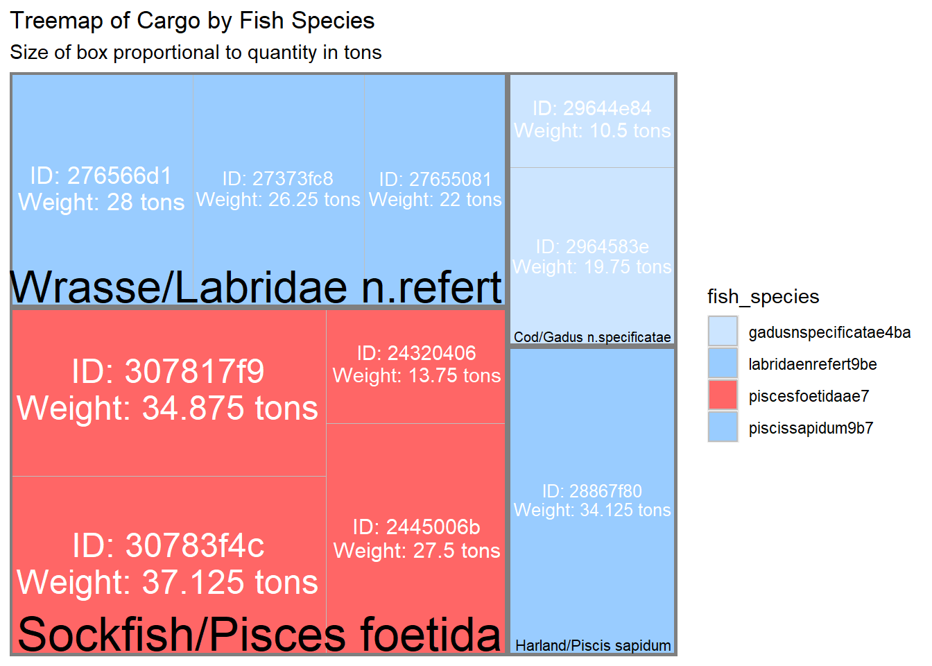
Exploring the associated cargo with SSEC, we observed 10 cargos mapped to Snapper Snatcher, with an alarming illegal catch of Sockfish/Pisces foetida, likely arising from its overstay in Ghoti Preserve.
There are no matches returned for Roach Robber which is unreasonable. This points to possibility of not reporting catches at the ports, or possibility of transhipment arrangement with other vessels, which is to be further explored.
Code
fish_species_color <-c("piscesfoetidaae7"="#FF6666", "piscisosseusb6d"="#FF9999", "piscessatisb87"="#FFCCCC", "gadusnspecificatae4ba"="#CCE5FF", "piscissapidum9b7"="#99CCFF", "habeaspisces4eb"="#66B2FF", "piscesfrigus900"="#CCE5FF", "oncorhynchusrosea790"="#FFCD00", "labridaenrefert9be"="#99CCFF", "thunnininveradb7"="#66B2FF")fish_species_labels <-c("gadusnspecificatae4ba"="Cod/Gadus n.specificatae", "piscesfrigus900"="Birdseye/Pisces frigus", "piscesfoetidaae7"="Sockfish/Pisces foetida", "labridaenrefert9be"="Wrasse/Labridae n.refert", "habeaspisces4eb"="Beauvoir/Habeas pisces", "piscissapidum9b7"="Harland/Piscis sapidum", "thunnininveradb7"="Tuna/Thunnini n.vera", "piscisosseusb6d"="Offidiaa/Piscis osseus", "piscessatisb87"="Helenaa/Pisces satis", "oncorhynchusrosea790"="Salmon")mapped_cargo_SSEC <- nearest_tx_date %>%filter(vessel_id %in%c("snappersnatcher7be", "roachrobberdb6")) %>%mutate(cargo_label =paste0("ID: ", sub("cargo_2035_", "", cargo_id), "\nWeight: ", qty_tons, " tons"), fish_species_label = fish_species_labels[fish_species])# Create the treemap plottreemap_plot <-ggplot(mapped_cargo_SSEC, aes(area = qty_tons, fill = fish_species, label = cargo_label,subgroup = fish_species_label)) +geom_treemap() +geom_treemap_subgroup_border() +geom_treemap_text(colour ="white", place ="centre", grow =TRUE) +geom_treemap_subgroup_text(aes(label = tx_date), colour ="black", place ="bottomright") +scale_fill_manual(values = fish_species_color) +labs(title ="Treemap of Cargo by Fish Species", subtitle ="Size of box proportional to quantity in tons")# Print the plotprint(treemap_plot)
 Trajectory until 14th of May.png)
 Dwell Time until 14th of May-01.png)
 Trajectory until 12th of May.png)